🥷 [S2] Challenge 13

Just KNIME It, Season 2 / Challenge 13 reference

Challenge question

Challenge 13: Rumour of Crime Rate

Level : Medium

Description: You ara a data scientist working for a real estate company, and heard a rumour that the "average number of rooms per dwelling" (RM) may be connected to the "per capita crime rate" (CRIM) depending on the city/town. You then decide to investigate if this is the case for Boston, the city where you live and work from. To this end, you decide to experiment with a machine learning regression model and with a topic that you have recently been studying: XAI. How are RM and CRIM connected in Boston? Hint: Consider calculating the SHAP values of each independent feature using a SHAP loop. Hint 2: Consider using a dependence plot to verify how RM and CRIM are connected visually.

The Challenge is an intriguing topic that evokes rumors and speculation, much like real-life situations. To address this question, we have two possible approaches. The first involves analyzing variables related to the "per capita crime rate" (CRIM) from the dataset. Alternatively, we can investigate the rumor directly. In this case, we will use the latter method as it is more straightforward for this particular question.

Workflow

Dataset intro

Even though the introduction to the Boston Real Estate Data dataset was not provided, it can easily be located due to its widespread popularity.

Each record in the database describes a Boston suburb or town. The data was drawn from the Boston Standard Metropolitan Statistical Area (SMSA) in 1970. The attributes are defined as follows (taken from the UCI Machine Learning Repository):

• CRIM per capita crime rate by town
• ZN proportion of residential land zoned for lots over 25,000 sq.ft.
• INDUS proportion of non-retail business acres per town
• CHAS Charles River dummy variable (= 1 if tract bounds river; 0 otherwise)
• NOX nitric oxides concentration (parts per 10 million)
• RM average number of rooms per dwelling
• AGE proportion of owner-occupied units built prior to 1940
• DIS weighted distances to five Boston employment centres
• RAD index of accessibility to radial highways
• TAX full-value property-tax rate per 10 000 USD
• PTRATIO pupil-teacher ratio by town
• B 1000 (Bk - 0.63)^2 where Bk is the proportion of black people by town
• LSTAT % lower status of the population
• MEDV Median value of owner-occupied homes in $1000's

Quick Dataset Overview

As this is a well-known dataset, many people have already invested time in it. Therefore, we won't go through the same steps. Instead, we will examine pre-processing and exploratory data analysis (EDA) sections in existing notebooks on Kaggle. We will focus on EDA because our target differs from the notebook authors. We found that there is no missing data, which is great. Additionally, the distribution appears to be fine (source: https://www.kaggle.com/code/marcinrutecki/regression-models-evaluation-metrics#4.2-Boston-House-Prices), which is nice.

Machine Learning Interpretability is important

Because it helps us understand how a machine learning model is making its predictions or decisions. This is crucial for several reasons:

1. Trust: If we don't understand how a model is making its predictions, we may not trust it. If we don't trust it, we're unlikely to use it.
2. Bias: Machine learning models can be biased, and if we don't understand how they're making decisions, we may not be able to detect or address that bias.
3. Accountability: In some cases, we may need to be able to explain to others how a decision was made. If we can't do that, we may not be able to hold the model or the people who created it accountable.
4. Improvement: Understanding how a model is making its predictions can help us improve the model and make it more accurate or efficient. In short, Machine Learning Interpretability is important because it helps us build trust in machine learning models, detect and address bias, hold models and their creators accountable, and improve the models themselves.

Shap Introduction

The SHAP value is a method used in machine learning to explain the contribution of each feature to the final prediction of a model. It stands for "SHapley Additive exPlanations" and is based on the concept of Shapley values from cooperative game theory. Essentially, the SHAP value calculates the impact of each feature on the prediction by comparing the model output with and without that particular feature. This allows for a more nuanced understanding of how the model is making its predictions and can help identify which features are most important in determining the outcome. The SHAP value is a popular tool for interpreting complex machine learning models and can be used for tasks such as feature selection, model comparison, and identifying bias in the model.

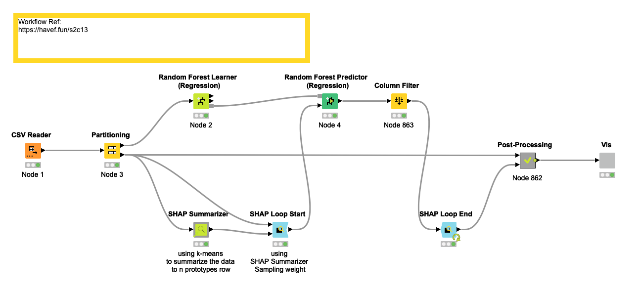
Our Workflow

We utilized 'Partitioning' node to divide the data into Dev and Test sets. To simplify our process, we opted not to consider more advanced machine learning algorithms, and instead, we used 'Random Forest'. Prior to running the 'SHAP Loop Start' node, we first used the 'SHAP Summarizer' node. Since the amount of data is relatively small, we chose to divide the data into twenty groups. Once the data segmentation was complete, we proceeded with the calculation of the SHAP value. Fortunately, the author of this Challenge provided us with a node called "Dependence Plot", which allowed us to easily analyze the SHAP value of the features and the relationship between RM and CRIM.

Analysis

The workflow is straightforward. Let's focus on the visualization component.

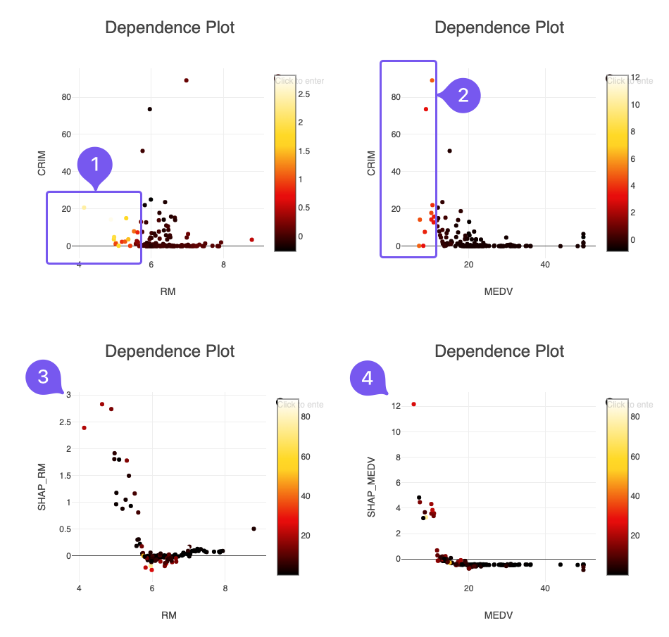
In the upper left figure, RM is on the horizontal axis, and CRIM is on the vertical axis. The color illustrates the SHAP value of RM. The brighter the point, the more significant its impact. It's apparent that for small RM values, their contribution to the crime rate is more pronounced. However, it's crucial to note that the crime rates associated with these values are not very high.

In the upper right figure, MEDV is on the horizontal axis, and the rest is the same as in the previous figure. MEDV refers to "Median value of owner-occupied homes in $1000's." Compared to RM, smaller MEDV values correspond to higher crime rates. Thus, RM is not a reliable single indicator of crime rates.

The lower left figure has RM on the horizontal axis and the SHAP value of RM on the vertical axis. The color represents the crime rate. It's evident that smaller RM values significantly contribute to the crime rate and smaller crime rates. This figure is similar to the upper left figure but viewed from a different angle.

The lower right figure doesn't require much explanation. The vertical axis is different from the lower-left figure's vertical axis ratio.

In conclusion, there is a correlation between RM and crime rates, but it is relatively weak, compared to the MEDV value.

Any thoughts?

• It may be more effective to analyze the raw data to identify factors that influence the crime rate
• To ensure the model's fairness, it may be necessary to exclude characteristics specifically related to Black People.
• Partial Dependence/ICE analysis should be considered.